[Econometrics] 5-2. Conditional Expectation Function

#regression_anatomy #CIA #OVB

조건부

CEF

???: 여러분 공부하는거,, 잘 생각해보시길 바랍니다!

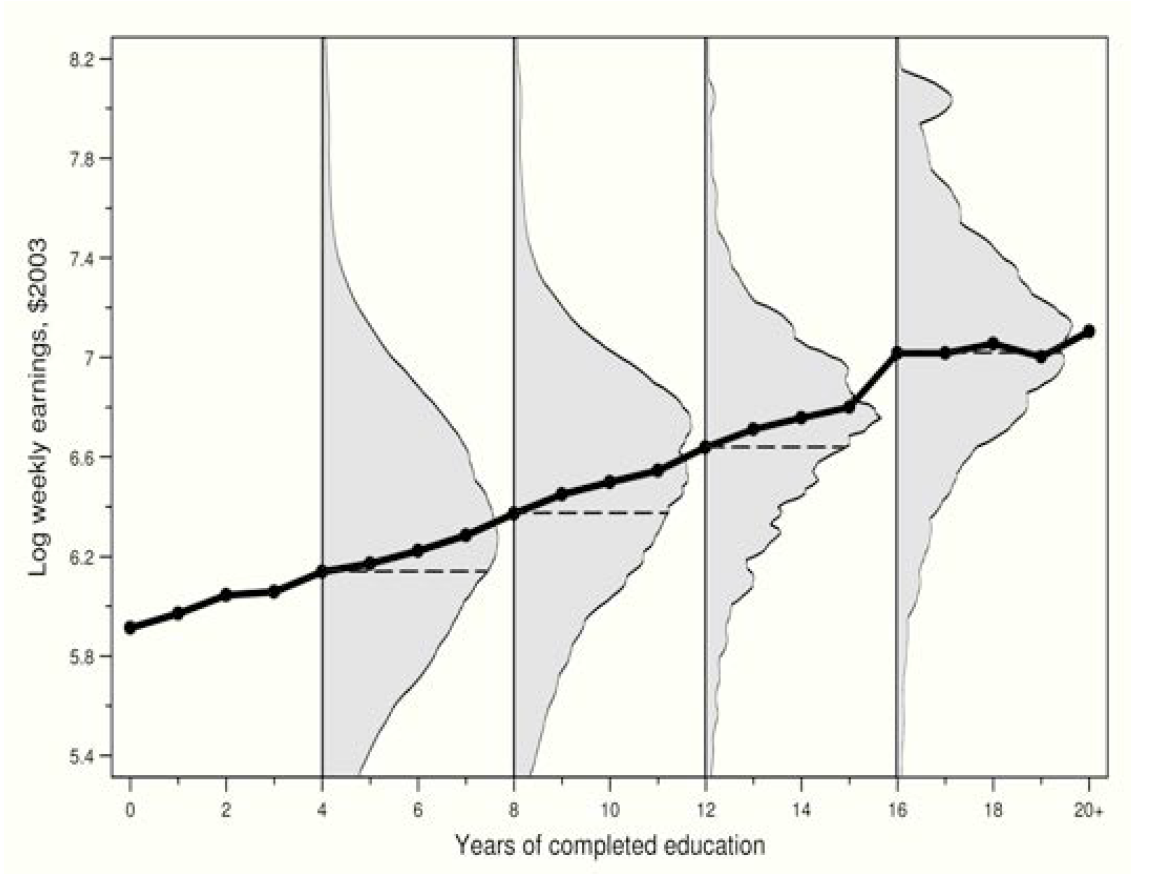
대표적인 CEF이다. 교육연수(X)에 따라 연봉 값(Y)이 달라지는, 즉 X에 따라 Y의 기댓값 E[Y]가 달라지는 $E[Y|X]$; CEF라고 볼 수 있다.

Properties of the CEF

결론은 linear CEF 짱짱맨

각 property의 인덱스는 AP의 수식 인덱스를 따름을 알립니다.

3.1.1. The CEF-Decomposition Property

Regression 상에서 Y는 곧 X로 1) 설명가능한 항과, 2) 그렇지 못한 항으로 Decomposed 된다는 것이다.

따라서, 그렇지 못한 항, 즉 error-term은 설명가능한 항과는 아무런 correlation이 없어야 하며, 이것은 곧 mean independent; uncorrelated를 의미한다.

\[\displaylines{\text{The CEF-Decomposition Property}\newline Y_i=E[Y_i|X_i]+\epsilon_i \newline \text{i) } \epsilon_i \text{ is mean independent of }X_i\,; E[\epsilon|X]=0 \newline \text{ii) }\epsilon_i \text{ is uncorrelated with any function of} X_i}\]

pf.

\[\displaylines{\text{i) }\quad \text{For}\quad Y=E[Y|X]+\epsilon \newline \text{Note, }\quad E[\epsilon|X]=0 \newline \text{Then, }\quad E[\epsilon|X]=E[Y-E[Y|X]|X]=E[Y|X]-E[Y|X]=0 \newline \newline \text{ii) }\quad \text{let }h(X_i) \text{ is a function of } X_i\newline E[h(X)\,\epsilon]=E\{h(X)\,E[\epsilon|X]\}=0, \;\text{since } E[\epsilon|X]=0}\]

3.1.2. The CEF-Prediction Property

Y를 설명하는 가장 좋은 Predictor로서의 X의 함수는 CEF라는 것이다; 여기서 ‘가장 좋은’이라 함은 MSE가 가장 작은 것을 의미한다.

\[\displaylines{\text{The CEF-Prediction Property}\newline E[Y|X]=arg\,min\,E[(Y-m(X))^2]\newline \text{i.e., the CEF is the minimum mean squared error (MMSE) predictor of }Y_i}\]

pf.

\[\displaylines{(Y-m(X))^2=((Y-E[Y|X])+(E[Y|X]-m(X)))^2\newline =(Y-E[Y|X])^2+2(Y-E[Y|X])(E[Y|X]-m(X))+(E[Y|X]-m(X))^2\newline\newline \text{The first and second term do not affect; while the last term be minimzed where}\; Y \;\text{equals}\; m(X)}\]

3.1.3. The ANOVA Theorem

3.1.1.의 연장선에서 Y의 분산은 1) X로 설명되는 항과, 2) Residual로 설명되는 항으로 Decompose될 수 있다는 Property이다.

두번째 항이 Residual이라는 것은 쉽게 유추할 수 있다. 분산의 정의를 고려할때, X로 설명되지 않았기 때문에 존재하는 잔차들의 분산이 $V(Y_i|X_i)$이기 때문.

\[\displaylines{\text{The ANOVA Theorem}\newline V(Y_i)=V(E[Y_i|X_i])+E[V(Y_i|X_i)]}\]

pf.

\[\displaylines{V(Y)=V(E[Y|X]+\epsilon)=V(E[Y|X])+V(\epsilon)\newline \text{Note, } E[Y|X] \text{ and } \epsilon \text{ are not correlated.} \\\\ \text{Then, the variance of } \epsilon \text{ is}\newline V(\epsilon)=E[\epsilon^2]=E[E[\epsilon^2|X]]=E[V[Y|X]] \quad \because E[\epsilon] = 0 \\\\ \text{Thus, }V(Y)=V(E[Y|X])+E[V[Y|X]]}\]

3.1.4. The Linear CEF Theorem

3.1.2.에서 우리는 Y를 예측(Predict)하는 가장 좋은 함수는 CEF라는 것을 보인 바 있다. 3.1.2. 식의 상에서 m(X)는 X와 관련된 어떠한 임의의 함수도 가능하지만, 우리는 X에 대한 linear function으로, 곧 X’b라는 단순한 모델로 접근해보고자 한다.

3.1.4. The Linear CEF Theorem는 즉 CEF가 선형함수라고 가정하면, 전체 population에 대한 regression function이 동일한 선형함수라는 것이다.

\[\displaylines{\text{The Linear CEF Theorem (Regression-justification I)}\newline \text{Suppose the CEF is linear; then the population regression function is it.}}\]

pf.

\[\displaylines{\text{Suppose } E[Y|X]=X'\beta^*;\newline \text{Since, } E[X(Y-E[Y|X])]=0 \text{ by CEF-Decomposition property (3.1.1)}\newline \text{Then, by substitution, } E[X(Y-E[Y|X])]=E[X(Y-X'\beta^*)]=E[XY-XX'\beta^*]=0\newline \text{Thus, } \beta^*=E[XX']^{-1}E[XY], \text{ which refers }\beta \text{ (the estimator for the population)}}\]

3.1.5. The Best Linear Predictor Theorem

Regression solves the population least squares problem and is therefore the BLP of Yi given Xi

즉, 전체 population에 대한 regression은 곧 반대로 CEF에게도 Best Linear Predictor라는 것이다.

\[\displaylines{\text{The Best Linear Predictor Theorem (Regression-justification II)}\newline \text{The function } X'\beta \text{ is the best linear predictor of }Y \text{ given } X \text{ in a MMSE Sense.}}\]

pf.

\[\displaylines{\beta \text{ is being defined for solving } arg\,\underset b min\,E[(Y-X'b)^2]\newline \beta=E[XX']^{-1}E[XY]\newline \text{Derivation of the }\hat\beta \text{ at the population regression would not be necessary.}}\]

3.1.6. The Regression-CEF Theorem

3.1.4.와 3.1.5.의 결과를 통해 우리는 Regression의 결과인 $\beta$가 CEF에 대해서도 가장 좋은 predictor임을 확인할 수 있다.

\[\displaylines{\text{The Regression-CEF Theorem (Regression-justification III)}\newline \text{The function } X'\beta \text{ provides the MMSE linear approximation to }E[Y|X],\text{ that is,}\newline \beta=arg\,\underset b min\,E\{(E[Y|X]-X'b)^2\}}\]

pf.

\[\displaylines{(Y-X'b)^2=\{(Y-E[Y|X])+(E[Y|X]-X'b)\}^2\newline =(Y-E[Y|X])^2+(E[Y|X]-X'b)^2+2(Y-E[Y|X])(E[Y|X]-X'b)\newline\newline}\] \[\displaylines{\text{The first term does not involve b, and the last term has expectation zero by CEF-decomposition property (3.1.2).}\newline \text{Thus, only second term has left, and the solution is same as the population least squares problem, which is,}\newline \beta=E[XX']^{-1}E[XY]\newline }\]

3.1.6. The Regression-CEF Theorem을 통해, Y라는 전체 population의 거대한 데이터 대신, $E[Y|X]$에 weightening으로 adjust만 해주면 정확히 동일한 $\beta$를 구할 수 있다는 것이다.

Regression Anatomy

Anatomy, 즉 Regression을 해부하는 narrow down을 시도하는 것이다.

Bivariate Reg.

\[\displaylines{min\underset{a,b} E{[Y_i-a-bx_i]^2}\newline\newline \text{by F.O.C.,}\; \alpha=E[Y_i-\alpha-bx_i]=0\newline \beta=E{[Y_i-\alpha-\beta x_i]x_i}=0\newline\newline \text{Thus,}\;\alpha=E[Y_i]-\beta E[X_i]\newline \beta=\frac{Cov(x_i,y_i)}{V(x_i)}}\]

Multi-variate Case

the k-th non-constant slope coefficient is:

\[\beta_k=\frac{Cov(Y_i,\tilde x_{ki})}{Var(\tilde x_{ki})}\]

where $\tilde x_{ki}$ is the residual from regressing $x_{ki}$ on all the other covariates.

Causality and Endogeneity

Regression이 인과관계에 대한 인사이트를 줄 수 있는가?

우리는 앞서 CEF가 MMSE 측면에서 population regression에 가장 좋은 설명력을 가진다는 것을 확인하였다.

하지만, 모든 Regression이 항상 인과관계를 설명해줄 수는 없을 것이다. 후술할 Endogeneity Issues 때문이다.

AP는 아래와 같이 설명하였다.

“the CEF is causal when it describes differences in average potential outcomes for a fixed reference population”

의역하면 곧, 동일 individual에 대해 treatment가 없고 있고의 차이가 비교된 값들의 평균이어야 하며, 즉 Selection bias가 없어야 한다는 것이다.

Endogeneity Issues는 다음과 같은 원인으로 발생할 수 있다.

• Omitted Variables (Bias)
  • Y에 영향을 주는 관측하지 못한 (unobservable) 변수가 regression이 포함되지 않았을때,
  • 그 상황에서 기존의 X와 correlation이 존재하면 곧 error term과 correlation이 발생하여 OVB가 발생한다.
• Measurement Error
• Simultaneity

최악은, 위의 세가지 이유가 배타적이라 아니라 전부 발생할수도 있다는 점이다.

OVB Example: The Returns to College

The classic example of treatment endogeneity in the labor literature is in measuring the returns to college (C_i=0,1)

\[\displaylines{ E[Y_i|C_i=1]-E[Y_i|C_i=0]=E[Y_{1i}|C_i=1]-E[Y_{0i}|C_i=0]\newline =E[Y_{1i}-Y_{0i}|C_i=1]+(\,E[Y_{0i}|C_i=1]-E[Y_{0i}|C_i=0]\,)\newline \equiv ATT +\text{ Selection Bias} }\]

대표적으로 발생할 수 있는 연봉과 학력 수준 사이의 regression 사이의 OV는 ability 이다.

ability는 직업과 연봉을 결정짓는 가장 중요한 변수중 하나라고 할 수 있지만, 측정의 어려움 등으로 인해 기존의 회귀식에서 빠진채 진행이 되었다.

그리고 단순한 추측으로 예컨데, 이번 regression 식에서의 측정된 Effect 크기인 ATT + Selection Bias에서는 둘 다 양의 값을 가질 것이라 예상해볼 수 있다.

\[\text{Selection Bias : }\;E[Y_{0i}|C_i=1]-E[Y_{0i}|C_i=0]>0\]

본 selection bias 항을 해석해보자면, C라는 조건에 따라, 즉 대학에 간 사람들과 대학에 가지 않은 사람들이, 만약 모두 대학에 가지 않았더라도 연봉의 차이는 존재할 것이라는 유추를 해볼 수 있다. 능력의 차이가 있기 때문이다.

조금더 설명을 붙여보자면, 학력이 높은 개인들은 능력 또한 높을 것이란 상관관계를 추측해볼 수 있다.

즉, 능력, ability는 Omitted Variable이다.

Conditional Independence Assumption (CIA)

At the Binary setting

\[\displaylines{\text{Randomized Experiment : }\;\{Y_{0i},Y_{1i}\}\perp\!\!\!\perp C_i\newline \text{CIA : }\;\{Y_{0i},Y_{1i}\}\perp\!\!\!\perp C_i|X_i}\]

CIA means that $C_i$ is “as good as randomly assigned,”conditional on $X_i$ , and thus the selection bias vanishes.

CIA는 오히려 the conditioning variables, $X_i$를 통제함으로써 (regression에 포함시킴으로써) $C_i$의 randomness를 충족시키고 이를 통해 Selection Bias를 제거한 Treatment Effect를 찾자는 것이다.

일종의 Fixed Effect라고 볼 수도 있다.

그렇다면 어떤 변수가 conditioning variables, $X_i$가 될 수 있을까?

Proxies for known omitted variables are obvious candidates.

보통 유관한 변수들을 추가한다. 예를 들어, 앞선 예시의 ability라는 측정하기 어려운 OV를 대신하여 X로 IQ를 일종의 프록시(간접변수)로 사용할 수 있을 것이다.

$C_i|X_i$가 Y와 독립이기 때문에 두번째 행에서 세번째로 넘어갈때에 제약이 없고, Selection Bias가 없는 Treatment Effect의 효과를 확인할 수 있다.

\[\displaylines{ E[Y_i|X_i,C_i=1]-E[Y_i|X_i,C_i=0]\newline =E[Y_{1i}|X_i,C_i=1]-E[Y_{0i}|X_i,C_i=0]\newline =E[Y_{1i}|X_i,C_i=1]-E[Y_{0i}|X_i,C_i=1]\newline =E[Y_{1i}-Y_{0i}|X_i,C_i=1]=E[Y_{1i}-Y_{0i}|X_i] }\]

직접 예시를 통해 해석해보자. 앞선 예시의 IQ를 controlling variable을 통제한다고 하자.

같은 IQ를 가진 참가자들이 대학을 가고 안가고는 취향 차이라는, Selection Bias를 최대한 통제한다고 볼 수 있을것이다.

따라서, 두번째 행에서 세번째로 넘어갈때, 대학을 가고 안가고는 IQ가 같은 사람들끼리는 큰 상관이 없기 때문에, 제약이 없다고 가정하며, 이를 통해 우리가 원하는 Treatment Effect를 포착할 수 있다는 것이다.

\[\text{ATT : }E\{E[Y_{1i}-Y_{0i}|X_i]|C_i=1\}=E[Y_{1i}-Y_{0i}|C_i=1]\]

IQ와 같이 각 controlling variable 값 별로 treatment effect가 통제된 개별 값이 있기 때문에, ATT는 곧 이에 대해 controlling variable에 대한 분포를 기반한 weigthened average를 통해 구할 수 있다.

조금 더 예를 막 나아가보면, IQ가 예를 들어 100을 평균으로 하는 일종의 정규분포를 따른다면, IQ 별 Treatment Effect를 나열하지 말고 정규분포를 토대로 전체 population의 Treatment Effect를 유추해볼 수 있다는 뜻이다.

Extending CIA to Non-Binary setting

Treatment가 항상 앞선 예시의 대학을 가고 안가고 처럼 0과 1로만 나누어져 있지는 않을 것이다.

예를 들어 변수가 교육 연수에 해당한다면, 0부터 일반적으로 12나 16 여기서 멈출걸 혹은 20+도 있을 것이다.

Extension에서 Potential outcomes는 아래와 같을 것이다. Extension들의 유도와 해석은 앞선 그것과 동일하다.

\[\displaylines{Y_{s,i}=f_i(s)\newline \text{Then, CIA: }\; Y_{si}\perp\!\!\!\perp s_i|X_i\quad \forall s}\] \[\displaylines{ E[f_i(12)|X_i,s_i=12]-E[f_i(11)|X_i,s_i=11]\newline =E[f_i(12)|X_i,s_i=12]-E[f_i(11)|X_i,s_i=12]\newline =E[f_i(12)-f_i(11)|X_i,s_i=12]=E[f_i(12)-f_i(11)|X_i] }\] \[\text{ATT : }E\{E[f_i(12)-f_i(11)|X_i]|s_i=12\}=E[f_i(12)-f_i(11)|s_i=12]\]

The Regression Context

\[\displaylines{Y_{s,i}=f_i(s)=\alpha+\rho s+\eta_i \newline \text{in the CIA: }\; Y_{si}\perp\!\!\!\perp s_i|X_i\quad \forall s \newline }\]

여기서 위 식의 error term인 $\eta$를 자세히 살펴보자 (decompose).

\[\displaylines{\eta_i=X_i'\gamma+\nu_i \newline \text{Then, } E[\eta_i|X_i]=X_i'\gamma, \text{ and } E[\nu_i|X_i]=0 \text{ by decomposition property}\\\\ \text{CIA implies: } E[Y_{s,i}|X_i, s_i]=E[Y_{s,i}|X_i]\newline =\alpha+\rho s+E[\eta_i|X_i]=\alpha+\rho s+X_i'\gamma \\\\ \text{Thus, } Y_i=\alpha+\rho s+X_i'\gamma+\nu_i \newline \text{satisfying }\; E[\nu_i|X_i,s_i]=0}\]

$\eta$는 OVB로 인해 X와 correlation이 있을수도 있고 없을 수도 있다.

첫번째 파트에서는 $\eta$를 따라서 decompose 하여 X로 설명가능한 부분(correlation 존재)과 그렇지 않은 부분으로 나누었을때를 보여주고 있는 것이다.

두번째 파트에서는 CIA는 X를 통제하기 때문에, 앞선 Y의 식을 유도하며 $\eta$를 X로 설명 가능한 파트만 남겨놓을 수 있다는 걸 보여주고 있다.

따라서 마지막 파트에서는 결국, X로도 설명할 수 없는 $\nu$를 남겨놓고 (mean independence 만족) Y를 X에 대해 완벽하게 decompose할 수 있다는 것을 보이고 있다.

결론적으로, CIA를 통해 기존의 s 뿐만 아니라 X 또한 regression에 포함시켜 진행하면, OVB를 최대한 control 해볼 수 있다는 것이다.

Omitted Variables Bias (OVB)

\[\displaylines{Y_{i}=\alpha+\rho s_i+A_i'\gamma +\epsilon_i \newline \text{by Regression Anatomy, }\;\frac{Cov(Y,s)}{Var(s)}=\rho+\gamma'\delta_{As}\\\\ \frac{Cov(Y,s)}{Var(s)}=\frac{Cov(\alpha+\rho s_i+A_i'\gamma +\epsilon_i, \; s_i)}{Var(s)}\newline =\frac{\rho Var(s)}{Var(s)}+\frac{\gamma' Cov(A, s)}{Var(s)}\equiv\rho+\gamma'\delta_{As} }\]

where $\delta_{As}$ is the vector of coefficients from regressions of the elements of A on s

$\rho$만 있어야하는 기본 anatomy에서, $\gamma’\delta_{As}$ 항이 추가 되었다. 이것이 OVB라고 할 수 있다.