[Econometrics] 3. Multiple Choice

#Multinomial_logit #Conditional_logit #IIA #Nested_logit #Mixed_logit #Probit #Ordered_Response

한식 양식 일식 중식, 그것이 multiple choice다.

Multiple Choice

Multinomial Response

Y takes values in a finites set,

\[Y\in \{1,2,...,j\}\]

선택가능한 옵션들은 alternatives라고 부른다.

예를 들어, 한 개인이 서울에서 부산으로 가고자 할 때, 고를 수 있는 옵션은 1: 비행기, 2: 기차, 3: 자가용, 4: 도보(?) 등이 있을 것이다.

각자 생각하는 유틸리티, The utility of alternative j를 생각해볼 수 있을 것이다.

\[U_j^*=X'\beta_j+\epsilon_j\]

여기서 $\epsilon_j$는 individual-specific, and contains unobserved factors 들을 포함하는 에러텀이다.

이렇게 정의된 각 alternative의 utility를 기반으로 사용자의 선택을 예측하는 것은 곧,

\[Y=j,\;if\;U^*_j \geq U^*_l\;(for\;all\;l)\]

다른 어떤 alternatives의 utility보다 j의 utility가 높음을 의미한다.

Location of $\beta_j$ cannot be identified

앞서 multinomial choice의 alternative가 선택되는 것은 다른 alternatives와의 상대적인 비교를 통해 가장 높은 utility의 alter가 선택되는 것임을 알 수 있었다.

그렇기 때문에, 곧, $\beta_j$의 절대적인 위치 (location)는 알 수 없다는 것을 뜻하기도 한다.

또 다른 의미로는, 개개인의 특성계수값을 모아놓은 X에 대하여 어떤 상수 $\gamma$를 곱해 더하거나 빼는 것(혹은 전체 utility에 상수를 곱하거나)은 모든 alternative에 동일하게 적용된다 할 때에, 선택에 영향을 줄 수 없음을 뜻한다.

따라서, 우리는 모델을 초기 생성하여 디자인하는데에 있어선, locations들을 normalization 시켜줄 필요성을 느낀다.

첫번째 내지 마지막 번째 등, 특정 alternative의 location을 0으로 함에 따라 normalization을 할 수 있을 것이다.

Models

Multinomial Logit

\[P_j(x)=\frac{exp(x'\beta_j)}{\Sigma \,exp(x'\beta_l)}\]

alternatives가 두 개 뿐일때, 위의 식은 다시금 binary model의 logit model의 식과 동일하다는 것을 알 수 있다.

ㄴLikelihood

곧바로 likelihood에 대해서도 derive를 해보자.

Y의 prob mass function은 아래와 같다.

\[\displaylines{\pi(Y|X,\beta)=\Pi\, P_j(X|\beta)^{1\{Y=j\}}\newline l_n(\beta)=\Sigma\Sigma\, 1\{Y_i=j\}\,log\,P_j(X_i|\beta)\newline \hat\beta=arg\,max\,l_n(\beta)}\]

본 $\beta$ estimator는 손으로 구할 수 없기 때문에, Stata 상에서는 numerical 한 방법으로 $\hat\beta$를 구해준다.

ㄴMarginal Effect

\[\text{marginal effect}\; :\;\frac{\partial}{\partial x}P_j(x)=P_j(x)\,(\beta_j-\Sigma\,\beta_lP_l(x))\]

Derivation)

\[\displaylines{P_j(x)=\frac{exp(x'\beta_j)}{\Sigma \,exp(x'\beta_l)}=\frac{exp(x'\beta_j)}{A}\newline \frac{\partial P_j(x)}{\partial x}=\beta_j exp(x'\beta_j)A^{-1}-exp(x'\beta_j)A^{-1}\Sigma exp(x'\beta_l)\beta_l A^{-1}\newline =\beta_jP_j-P_j\Sigma P_l\beta_l\newline =P_j(\beta_j-\Sigma \beta_l P_l)}\]

Conditional Logit

교통수단의 비용, 소요시간 등 각각의 alternative 별로 또 다른 attributes들은 어떻게 처리할 것인가? (기존의 multinomial logit의 X는 개개인의 attributes들로 이루어진 벡터였음을 상기하자)

새로이 우리는 alternative-specific regressors를 적용시켜보며, 이를 Conditional Logit Model의 이름으로 발전되어왔다 (McFadden, 1970).

Conditional logit에서는 앞서 언급한 alternative j 별로 다른 특징들을 X에 모두 반영하여 아래와 같은 식을 전개한다.

\[U_j^*=X_j'\gamma+\epsilon_j\]

기존의 Multinomial logit과 차이를 비교했을때, Multinomial logit에서는 alternative 별로 $\beta_j$가 달랐다면, Conditional logit에서는 개별 $X_j$가 다르며 $\gamma$는 alternative에 관계 없이 동일하게 유지되는 것을 알 수 있다.

이를 혼용하면 일반적인 아래와 같은 logit 식을 얻을 수 있다.

allows some regressors X_j to vary across alternatives while other regressors W do not vary across j

\[\displaylines{U_j^*=W'\beta_j'+X_j'\gamma+\epsilon_j \newline \epsilon_j \sim \text{ Type 1 Extreme Value}=exp(-exp(-\epsilon))}\]

ㄴ Likelihood

\[\displaylines{For \quad P_j(w,x)=\frac{exp(w'\beta_j+x_j'\gamma)}{\Sigma \,exp(w'\beta_l+x_l'\gamma)}\newline\newline let \quad \theta=(\beta_1,\beta_2,...,\beta_j,\gamma) \newline then,\quad l_n(\theta)=\Sigma\Sigma\, 1\{Y_i=j\}\,log\,P_j(W_i,X_i|\theta)\newline \hat\theta=arg\,max\,l_n(\theta)}\]

본 $\theta$ estimator 또한 손으로 구할 수 없기 때문에, Stata 상에서는 numerical 한 방법으로 $\hat\theta$를 구해준다.

ㄴMarginal Effects

\[\displaylines{ \delta_{jj}(w,x)= \frac{\partial}{\partial x_j}P_j(w,x)=\gamma P_j(w,x)\,(1-P_j(w,x))\newline \delta_{jl}(w,x)= \frac{\partial}{\partial x_l}P_j(w,x)=-\gamma P_j(w,x)P_l(w,x)\newline \newline AME_{jl}=E[\delta_{jl}(W,X)] }\]

Derivation)

\[\displaylines{ P_j(w,x)=\frac{exp(w'\beta_j+x_j'\gamma)}{\Sigma \,exp(w'\beta_l+x_l'\gamma)}=\frac{exp(w'\beta_j+x_j'\gamma)}{A}\newline\newline \delta_{jj}(x)=\frac{\partial P_j(w,x)}{\partial x_j}\newline =\gamma exp(w'\beta_j+x_j'\gamma)A^{-1}-exp(w'\beta_j+x_j'\gamma)A^{-2}exp(w'\beta_j+x_j'\gamma)\newline =\gamma P_j -P_j^2\gamma =\gamma P_j(1-P_j)\newline\newline \delta_{jl}(x)=\frac{\partial P_j(w,x)}{\partial x_l}\newline =-exp(w'\beta_j+x_j'\gamma)A^{-1}exp(w'\beta_l+x_l'\gamma)\gamma A^{-1} \newline =-\gamma P_jP_l }\]

Independence of Irrelevant Alternatives

Multinomial / Conditional Logit을 사용하는데에 있어 굉장한 threat이 존재하는데, 이는 Independence of Irrelevant Alternatives의 문제이다.

IIA

서로 다른 두 옵션(alternatives)가 선택될 확률의 상대적인 비율을 계산해보자.

\[\frac{P_j(W,X)}{P_l(W,X)}=\frac{exp(W'\beta_j+X_j'\gamma)}{exp(W'\beta_l+X_l'\gamma)}\]

위 식의 값을 결정짓는 변수들은 오롯이 j번째 alternative와 l번째 alternative의 특징들로만 구성 되어있는 것을 확인할 수 있다.

예를 들어 j를 예시의 자동차, l을 기차라고 하자.

하지만 만약 다른 alternative인 k: 비행기의 가격(X_k)이 변화한다고 하자.

이 비행기 가격의 변화가 j와 l의 alternative에 절대적으로 영향을 끼치지 않는다고 단언할 수 있을까? 아니다; 이것이 IIA이다.

IIA를 해결하기 위한 발전된 model 들을 알아보자.

Nested Logit

이에 대응하는 해결방안 (중 하나)은 alternatives 간에 그룹을 지어주는 것이다. 아래의 그림이 예시가 될 것이다.

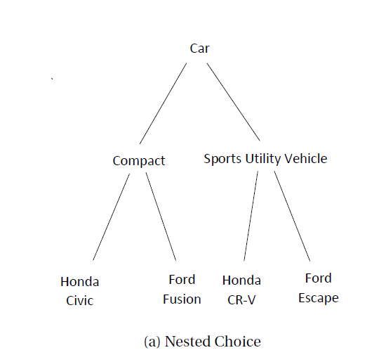
J groups each with $K_j$ alternatives 라고 일반적인 note가 이루어진다.

\[U_{jk}^*=W'\beta_{jk}'+X_{jk}'\gamma+\epsilon_{jk}\]

곧, Nested Logit의 Utility 식은 위와 같이 먼저 j번째 그룹에 대한 아래첨자가 추가되고 그 뒤에 k번째 alternative index가 추가된다고 볼 수 있겠다.

본 모델에서 각 groups 간의 correlation은 없다고 가정한다.

대신, 각 group 내의 alternatives들의 correlation은 dis-similarity parameter, $\tau_j$로 표현된다.

만약, $\tau_j=1$이라면, 이는 곧 그룹 내의 alternatives 간 correlation이 없기 때문에 기존의 conditional logit를 따른다는 것을 의미한다.

모델을 디자인 할 때, 기존의 logit 모델처럼 location의 정규화를 위한 특정 alternative의 location을 0으로 맞춰주는 작업이 필요하다.

Alternatives with a high(low) degree of substitutability should be placed in the same(different) group.

\[\text{Response Probability}:\;P_{jk}=P_{k|j}P_j\]

Response Prob은 위와 같은데, 이는 곧 j개의 그룹 중 하나를 선택하고, 그 그룹 내의 k개의 alternatives 중 하나를 고른다는 것을 의미한다고 볼 수 있다.

ㄴLimitations

Typically, there is not a unique obvious structure; consequently any proposed grouping is subject to mis-specification

Mixed Logit

Generalization of the conditional logit which allows the coeff on the alternative varying regressors to be random across individuals

개별 소비자들이 각 alternative의 특성에 갖는 가중치, 인지하는 중요도 등이 다 다른 것을 반영하고자 하는 모델이다.

예를 들어 어떤 소비자는 자동차라는 alternative를 볼때 연비를 중요하게 볼 수도 있고, 다른 소비자는 좌석수를 중요하게 볼 수도 있으며, 비행기라는 alternative에 대해 가격을 중요하게 볼 수도 있고, 보딩 서비스에 대해 중요하게 생각하는 소비자도 있을 것이다. 즉 $\gamma$가 일정하지 않고, random하다는 뜻이다.

\[\displaylines{U_{j}^*=W'\beta_{j}'+X_{j}'\eta+\epsilon_{j},\quad \eta\sim N(\gamma, \Sigma)\newline =W'\beta_{j}'+X_{j}'\gamma+X'_j(\eta-\gamma)+\epsilon_{j}\newline =W'\beta_{j}'+X_{j}'\gamma+v_j}\]

Mixed Logit의 기본 수식은 기존의 conditional logit과 다르지 않다. 하지만 $\eta$를 평균값의 $\gamma$ 항과 그렇지 않은 error-term 항으로 분리하여 새로운 error term $v_j$를 만들었는데, 이 $v_j$의 기댓값을 유도해보자.

\[\displaylines{E[v_jv_l|X_j,X_l]=E[X_j'(\eta-\gamma)(\eta-\gamma)'X_l|X_j,X_l]\newline =X'_j\,Var(\eta)\,X_l}\]

방금 위의 non-zero correlation은 곧 IIA 문제에 발생하지 않는 것을 뜻하고, 이는 곧 mixed logit이 conditional logit보다 소비자들의 선택 양식을 설명하는데 있어 더 유연성(flexibility)을 갖음을 뜻한다고 할 수 있다.

Probit model

logit 분포와 달리, $\epsilon$이 정규분포를 따르는 차이 말고 다른 큰 차이는 없다. IIA property 마저 동일하지 않지만 거의 유사하게 발생한다고 한다.

하지만 logit에 비해 computational power에 많은 의존성을 띄기 때문에, 무조건적으로 선호되거나 많이 사용되지는 않는 지금이라고 한다.

Ordered Response

Y가 ordinal (ordered) interpretation의 종속변수일 때는 어떠할까?

예를 들어 교수님의 강의평가를 할때 5점척도 중 한가지 점수 (1,2,3,4 or 5)를 골라야한다면; 이는 기존의 multinomial response와는 결이 다른 선택양식일 것이다.

위와 같이 각 $\alpha$ 값들 사이사이 범위에 따라 받는 점수가 순서대로 정해져있는 특징을 최대한 살리는것이 현실 반영을 많이 할 수 있는 좋은 모델이라 할 수 있을 것이다.

\[\displaylines{U^*=X'\beta+\epsilon\newline \epsilon \sim G}\]

​ Ordered Response의 특징은 $U^*$라는 latent continuous response에 대해, 각 범위에 따라 discrete한 점수로 모여진다는 것이다 (discretized version).

Response Prob. and Marginal Effect

\[\displaylines{P_j(x)=P[\alpha_{j-1}<U^*\leq \alpha_j|X=x]\newline =G(\alpha_j-X'\beta)-G(\alpha_{j-1}-X'\beta)\newline \newline Thus,\quad P[Y\leq j|X=x]=G(\alpha_j-X'\beta)}\] \[\text{marginal effect}\;:\frac{\partial}{\partial x}P_j(x)=\beta(g(\alpha_j-X'\beta)-g(\alpha_{j-1}-X'\beta))\]